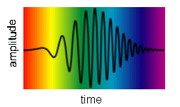
A sinusoidal plane wave extends to infinity in space and time.  It is perfectly coherent in space and time, its coherence length, coherence time, and coherence area are all infinite.  All real waves are wave pulses, they last for a finite time interval and have finite extend perpendicular to their direction of propagation.  They are mathematically described by non-periodic functions.  We therefore have to learn how to analyze non-periodic functions to find the frequencies present in wave pulses to determine Δω and the coherence length.

The light pulse in the figure above contains many frequencies. To determine the coherence length, we need to know its frequency content.

Any set of sinusoidal waves whose frequencies belong to a harmonic series will combine to produce a periodic complex wave, whose repetition frequency is that of the series fundamental.  The individual components may have any amplitudes and any relative phases.  These amplitudes and phases determine the shape of the complex waveform.

According to Fourier analysis, an arbitrary periodical waveform can be regarded as a superposition of sinusoidal waves.  Fourier synthesis means superimposing many sinusoidal waves to obtain the arbitrary periodic waveform.

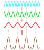
Any set of sinusoidal waves whose frequencies do not belong to a harmonic series will combine to produce a complex wave that is not periodic.  Any non-periodic waveform may be built from a set of sinusoidal waves.  Each component must have just the right amplitude and relative phase to produce the desired waveform.

The Fourier series

Any piece-wise regular periodic function (finite # of discontinuities, finite # of extreme values) can be written as a series of imaginary exponentials.  Assume f(t) is a periodic function of t with fundamental period T = 1/f.

f(t) = ∑_-∞^+∞C_nexp(iω_nt)

Here ω_n = n2πf, Δω = ω_n+1 - ω_n = 2πf.  The coefficients C_m are given by

C_m = (1/T)∫₀^Tf(t)exp(-iω_mt)dt.

Using e^iωt = cos(ωt) + i sin(ωt) we can also write

f(t) = A₀/2 + ∑_n=1^∞ A_ncos(ω_nt) + ∑_n=1^∞ B_nsin(ω_nt)

with

A₀ = (2/T)∫₀^Tf(t)dt,  A_m = (2/T)∫₀^Tf(t)cos(ω_mt)dt,  B_m = (2/T)∫₀^Tf(t)sin(ω_mt)dt.
We have A_n = (C_n + C_-n), B_n = i(C_n - C_-n), A₀ = 2C₀,  n > 0.

Fourier's theorem states that any periodic function with period T (or spatial period or wavelength L) can be synthesized by a sum of harmonic functions whose periods (wavelengths) are integral submultiples of T (or L), such as T/2, T/3, ..., (or L/2, L/3, ...).

Synthesizing a square wave

Link:  Fourier Series Simulation

The Fourier transform

In the limit  T --> ∞ Fourier's theorem can be generalized to

f(t) = (1/(2π)^1/2)∫_-∞^+∞ f(ω)exp(iωt)dω 
f(ω) = (1/(2π)^1/2)∫_-∞^+∞ f(t)exp(-iωt)dt

Here f(t) and f(ω) are Fourier transforms of each other.

[Assume f(t) is a periodic function with period T.
f(t) = ∑_n=-∞^+∞ C_nexp(iω_nt) .
C_n = (1/T)∫₀^Tf(t)exp(-iω_nt)dt = (1/T)∫_-T/2^T/2f(t)exp(-iω_nt)dt.
Using Δω  = 2πf, Δω/(2π) = f = 1/T, we write
C_n = (Δω/(2π))∫_-T/2^T/2f(t)exp(-iω_nt)dt.

f(t) = (1/(2π))∑_n=-∞^+∞[exp(iω_nt)Δω ∫_-T/2^T/2f(t')exp(-iω_nt')dt'].
As T --> ∞ , Δω --> 0, and this becomes
f(t) = (1/(2π))∫_-∞^+∞exp(iω_nt)dω ∫_-∞^+∞f(t')exp(-iω_nt')dt'.

Defining f(ω) = (1/(2π)^1/2)∫_-∞^+∞ f(t)exp(-iωt)dt
we have f(t) = (1/(2π)^1/2)∫_-∞^+∞ f(ω)exp(iωt)dω.]

Note:  A Fourier transform is a linear transform.

f(t) = c₁f₁(t) + c₂f₂(t)  implies  f(ω) = c₁f₁(ω) + c₂f₂(ω).

Examples:

(a)  The Fourier transform of a rectangular pulse:

(b) The Fourier transform of a harmonic wave train of finite length:

Let f(t) = Aexp(iω₀t), -T₁/2 < t < T₁/2.
The width of the wave train in time is T₁.

f(ω) = (1/(2π)^1/2)∫_-∞^+∞ f(t)exp(-iωt)dt
= (A/(2π)^1/2)∫_-T1/2^T1/2 exp(-i(ω-ω₀)t)dt.

f(ω) = (A/((2π)^1/2i(ω-ω₀)))[exp(i(ω+ω₀)(T₁/2)) - exp(-i(ω-ω₀)(T₁/2))]
= (AT₁/(2π)^1/2)sin[(ω-ω₀)(T₁/2)]/(ω-ω₀)(T₁/2)
= (AT₁/(2π)^1/2)sin(u)/u,
with u = (ω-ω₀)(T₁/2).

f(ω) is a representation of the wave train in frequency space.  It gives the amplitudes and phases of the harmonic waves of all possible frequencies needed to synthesize the wave train.

The function sin(x)/x = sinc(x) is called the sinc function.

While it is not zero  for |x| > some number, we find that it has a dominant peak between x = -π and x = π with smaller fringes on the sides.
The major contributions to f(ω) sinc[(ω-ω₀)(T₁/2)] therefore come from the region
-π < (ω - ω₀)(T₁/2) < π, or  -2π < (ω - ω₀)T₁ < 2π.
If we define Δω = (ω - ω₀) as the width of the wave train in frequency space and Δt = T₁/2 as its width in time, then ΔωΔt = 2π, ΔfΔt = 1.

Uncertainty principle for wave packets: ΔfΔt ~ 1.
The frequency bandwidth is of the same order as the reciprocal of the temporal extend of the pulse.